Money as a Control System

New to control systems, or need a refresher? Start with Control Systems: A Primer.

I'm a controls engineer, so when I sat down to decide how money should move between my paycheck, my savings and my businesses, I drew it as a plant and a controller. The model is small, but it settles questions that are hard to argue about in words: where a dollar does the most work, how big a cash buffer needs to be, and when it is safe to put more capital into a business.

The system has three stages:

Stage	What it is	Control behavior
Storage	Long-term savings in a T-bill fund	A slow integrator with a small positive pole
Buffer	A checking account held at a fixed balance	A setpoint regulator that absorbs spending disturbances
Business	The holding company's ad-driven businesses	A high-gain stage with positive feedback through advertising

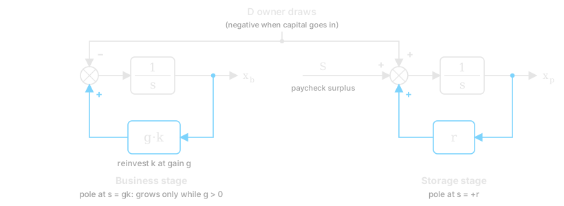
Figure 1. The two stages as positive-feedback integrators, coupled by owner draws D. Feedback paths are in blue.

1. The storage stage: a slow, unstable pole you want

Let $x(t)$ be the savings balance, $r$ the after-tax yield, and $u(t)$ the net inflow (surplus from each paycheck, plus owner draws from the business, minus any capital I put back in):

$$\frac{dx}{dt} = r\,x + u(t)$$

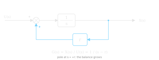
Figure 2. Storage: an integrator with positive feedback r, which puts the pole at s = +r.

Taking the Laplace transform:

$$X(s) = \frac{x_0}{s - r} + \frac{U(s)}{s - r}, \qquad G(s) = \frac{X(s)}{U(s)} = \frac{1}{s - r}$$

The pole sits at $s = +r$, in the right half-plane. In any other control problem that is the definition of unstable: the state grows without bound. For savings, that is exactly the behavior you want, and it is the cleanest way I know to state why compounding works.

For a constant net inflow $S$, the solution is:

$$x(t) = \left(x_0 + \frac{S}{r}\right)e^{rt} - \frac{S}{r}$$

The useful thing is how slow this pole is. At about 3% after tax, the doubling time is $\ln 2 / r \approx 23$ years. For the first decade the $e^{rt}$ term barely moves, and the balance is almost entirely the integral of $u$. Early on, the lever is the input, not the yield. Chasing an extra quarter point of yield is noise next to raising $S$.

2. The buffer stage: a regulator at a setpoint

The storage stage has dead time. Selling a fund and landing cash takes a few business days, which in the transfer function is a delay term $e^{-sT}$. Spending, on the other hand, happens instantly. Put a delayed source directly behind an instantaneous load and you get a supply gap every time spending spikes.

The fix is the same one you use on a production line: a buffer between the two. A checking account sits between spending and storage, held at a setpoint $x^*$. At each paycheck $k$, the controller tops it up by exactly what was used:

$$u[k] = x^* - x[k]$$

With spending $w[k]$ drawn down during the period, the buffer obeys:

$$x[k+1] = x[k] + u[k] - w[k] = x^* - w[k]$$

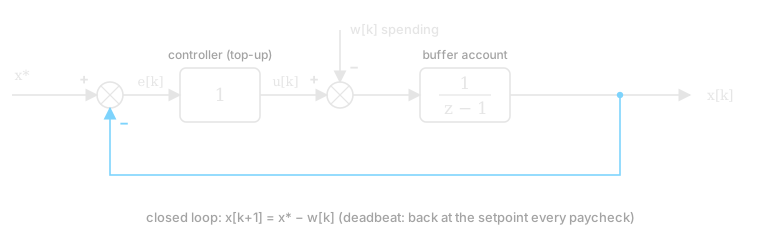
Figure 3. The buffer regulator. Spending enters as a disturbance, and the top-up controller returns the balance to x every paycheck.*

That is a deadbeat controller: any disturbance is fully corrected at the next sample, with no carried-over error and no oscillation. Sizing follows from the delay. The setpoint has to cover the largest spending surprise that can arrive before storage can respond:

$$x^* \geq \max_{\text{over } T} w$$

This is the same reasoning as buffer sizing in my manufacturing circuit model: a buffer exists to cover a rate mismatch for as long as the slower side takes to react.

3. The business stage: positive feedback through ads

The holding company spends on advertising, and some of that spend comes back as revenue. That return path makes it a feedback loop. Per dollar of ad spend $E$:

• revenue is $\text{ROAS} \cdot E$
• a fraction $\tau$ of revenue is reserved for taxes
• the spend itself costs $(1 - c_b)E$, where $c_b$ is the cashback the company's card returns

The net cash produced per ad dollar is the loop gain:

$$g = \text{ROAS}\,(1 - \tau) - (1 - c_b)$$

The business stage grows when $g > 0$ and drains when $g < 0$. Setting $g = 0$ gives the break-even:

$$\text{ROAS}^* = \frac{1 - c_b}{1 - \tau}$$

With a 30% tax reserve and 2% cashback, $\text{ROAS}^* = 0.98 / 0.70 = 1.40$. That is the cash-flow break-even, because the reserve is taken on gross revenue. Taxes are really owed on profit, so the true-profit break-even is lower, at $\text{ROAS} > 0.98$. The reserve on gross acts as damping: it holds back cash the loop could otherwise reinvest. That's sensible while revenue is uncertain. Once there is steady revenue, reserving on profit instead speeds the loop up.

4. Stability: the delay is the dangerous part

The gain $g$ is not something you know. You measure it, and the measurement arrives late. Ad platforms attribute conversions days after the spend, and payouts land days after that. So the real control problem is the controller that adjusts spend based on measured returns.

Suppose spend is adjusted each period toward the level where returns stop paying. Near that operating point, returns fall as spend rises, roughly $\text{ROAS}(E) \approx \text{ROAS}_0 - a\,(E - E_0)$. A controller that raises spend in proportion to how far measured ROAS sits above break-even, using a reading $d$ periods old, behaves like:

$$E[n+1] = E[n] - K a \,\big(E[n-d] - E_{\text{eq}}\big)$$

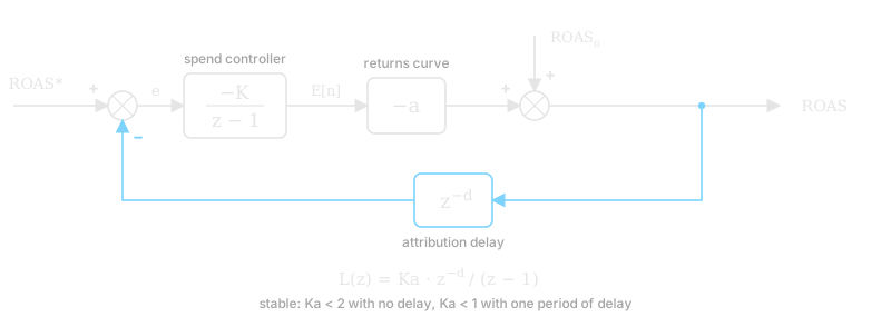
Figure 4. The ad spend loop. The attribution delay z⁻ᵈ in the feedback path is what limits the gain.

With no delay ($d = 0$), the characteristic root is $z = 1 - Ka$, which is stable for $0 < Ka < 2$. With one period of delay, the characteristic equation becomes $z^2 - z + Ka = 0$, and stability requires $Ka < 1$. Every period of delay tightens the limit on how aggressively you can react. Push past it and spend overshoots: you scale up on last week's good numbers, the returns come in worse, you cut hard, and the cycle repeats. That is the money version of a loop ringing because the dead time was ignored.

That gives the operating rule I actually follow, which is ordinary commissioning practice:

1. Identify the plant before closing the loop. Run ads at a fixed test budget, open loop, long enough to measure $g$ from real conversions.
2. Close the loop with a low gain. Add capital only while measured $g > 0$, in steps, waiting out the attribution delay between steps.
3. Watch for saturation. When ROAS falls toward break-even as spend rises, the stage has saturated. More input stops producing more output.
4. Rate-limit the actuator. Capital comes from paycheck surplus, never from debt or retirement money. That caps how fast the input can change and keeps a bad estimate from becoming a large loss.

5. Coupling the stages

The stages are in series. The business is the high-gain stage, and storage is the slow, durable one. Owner draws $D$ move money from the first to the second. The coupling rule follows from where each dollar does the most work:

• While the business stage has $g > 0$ and isn't saturated, keep $D$ low and let it reinvest. A dollar there earns $g$ per cycle, against $r$ per year in storage.
• Once it saturates, raise $D$. Extra money in a saturated stage earns nothing, and storage at least compounds.

It is the same logic as staging amplifiers: put the gain early, and don't feed a stage that has already clipped.

What the model leaves out

• Variance. $g$ is an average. A loop with a positive mean gain and a wide spread can still drain a small balance before the average shows up.
• Model error. The linearization around the operating point only holds nearby. That is one more reason to change spend in small steps.
• Taxes. The flat reserve is a simplification. The real rules are piecewise.

Even so, the model has earned its place. It turns "should I put more money into the business?" into a measurement question: what is $g$, how sure am I of it, and how long is the delay before I'll know if I'm wrong?

Related: Agent Autonomy as Loop Gain, which applies the same reasoning to how much an AI agent is allowed to do on its own.