Control Systems: A Primer

This page is the foundation for the rest of the Control Systems section. If you've never taken a controls course, or it's been a while, read this first. It covers just enough to follow Money as a Control System and Agent Autonomy as Loop Gain, and it uses the same notation as their diagrams. There's no proof here, only the ideas and the handful of equations that carry them.

1. Open loop and closed loop

Every control system has the same cast:

Part	What it does	Example: a room's heating
Plant $G$	The thing being controlled	The room
Controller $C$	Decides what to do	The thermostat logic
Actuation $u$	The controller's output, which drives the plant	Heater power
Output $y$	What you care about	Room temperature
Reference $r$	Where you want the output to be (the setpoint)	21 °C
Sensor $H$	Measures the output	The thermometer
Error $e$	Reference minus measurement	How far from 21 °C you are
Disturbance $d$	Anything outside that pushes the output	An open window

In an open-loop system, the controller sets the input and never checks the result. You run the heater for an hour and hope the room is warm. In a closed-loop system, the output is measured and fed back, and the controller acts on the error. That wire running from the output back to the input is what feedback means.

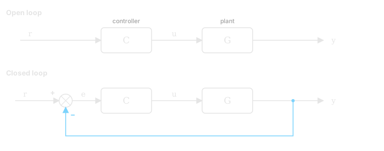
Figure 1. Top: open loop, where the output is never checked. Bottom: closed loop, where the output is fed back (blue) and subtracted from the reference.

2. Reading a block diagram

Block diagrams are the language of the field. The rules are few:

• A block multiplies its input by what's written inside it, the block's transfer function. Output $=$ (block) $\times$ input.
• A circle is a summing junction. Its inputs are added or subtracted according to the sign next to each arrow.
• A dot is a takeoff point: the same signal is copied onto two wires. A plain crossing with no dot means the wires aren't connected.
• The forward path runs left to right. The feedback path runs back underneath. On this site, feedback is drawn in blue.
• A diagonal arrow through a block means its gain is adjustable: something else tunes it. A dashed line is a slow, supervisory signal rather than one that changes every moment.

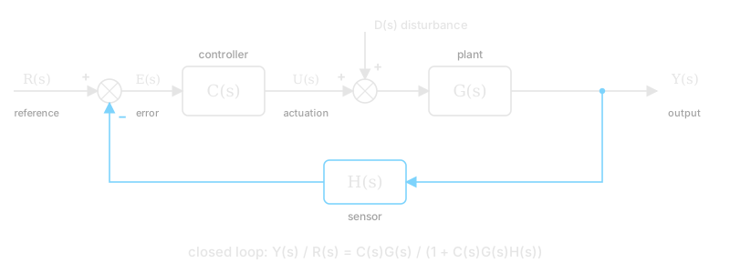
Figure 2. The standard feedback loop, with a disturbance entering at the plant input and a sensor in the feedback path.

Follow the signals in Figure 2 and two equations fall out: $E = R - HY$, and $Y = G\,(CE + D)$. Solve them together:

$$Y = \underbrace{\frac{CG}{1 + CGH}}_{\text{tracking}}\,R \;+\; \underbrace{\frac{G}{1 + CGH}}_{\text{disturbance}}\,D$$

The product $CGH$ is the loop gain, the total gain once around the loop. This one equation explains most of why feedback is worth having. When the loop gain is large, the first fraction approaches $1/H$, so the output follows the reference. The second fraction shrinks toward zero, so disturbances get pushed out. Feedback buys accuracy and robustness, and pays for it with the risk of instability, which the rest of this page is about.

The minus sign at the junction makes it negative feedback: the loop pushes against deviations. With a plus sign it becomes positive feedback, where the loop amplifies whatever it sees. That's dangerous in a thermostat, but it's exactly how compound interest and reinvested profit behave.

3. Transfer functions and the Laplace transform

The dynamics of a plant are usually differential equations. The Laplace transform turns them into algebra: a derivative becomes multiplication by $s$, and an integral becomes division by $s$. That's why every block in these diagrams is a fraction in $s$.

Element	Time domain	Transfer function	Everyday example
Gain	$y = k\,u$	$k$	A lever
Integrator	$\dot y = u$	$\dfrac{1}{s}$	A tank filling, a bank balance
First-order lag	$\tau \dot y + y = u$	$\dfrac{1}{\tau s + 1}$	A cup of coffee cooling
Dead time	$y(t) = u(t - T)$	$e^{-sT}$	A pipe: what goes in comes out $T$ seconds later

The integrator is the one to know. A bank balance is the integral of everything that flows in and out. A buffer on a production line is the integral of the difference between inflow and outflow. Any time something accumulates, there's a $1/s$ in the diagram.

4. Poles and stability

Write a transfer function as a fraction. The values of $s$ that make its denominator zero are its poles, and they decide how the system behaves. Each pole $p$ contributes a term like $e^{pt}$ to the response:

• A real pole $p < 0$ decays. The system settles.
• A real pole $p > 0$ grows without bound. The system is unstable.
• A complex pair $p = \sigma \pm j\omega$ oscillates at frequency $\omega$, decaying if $\sigma < 0$ and growing if $\sigma > 0$.

So the rule is geometric. Plot the poles in the complex s-plane: the system is stable when every pole is in the left half-plane.

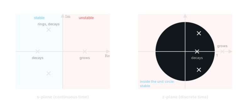
Figure 3. Left: in continuous time, poles in the left half-plane decay and poles in the right half-plane grow. Right: in discrete time, the boundary is the unit circle.

A quick example: $\dot x = r\,x$ has the transfer function $1/(s - r)$ and a pole at $s = r$. With $r > 0$, it grows exponentially. That's an unstable system in the textbook sense, and it's also a savings account. Whether "unstable" is bad depends on whether you wanted the thing to grow.

5. Damping and the step response

The standard way to see a system's character is its step response: change the reference suddenly and watch the output. Many real systems behave like a second-order system with a natural frequency $\omega_n$ and a damping ratio $\zeta$:

$$G(s) = \frac{\omega_n^2}{s^2 + 2\zeta\omega_n s + \omega_n^2}$$

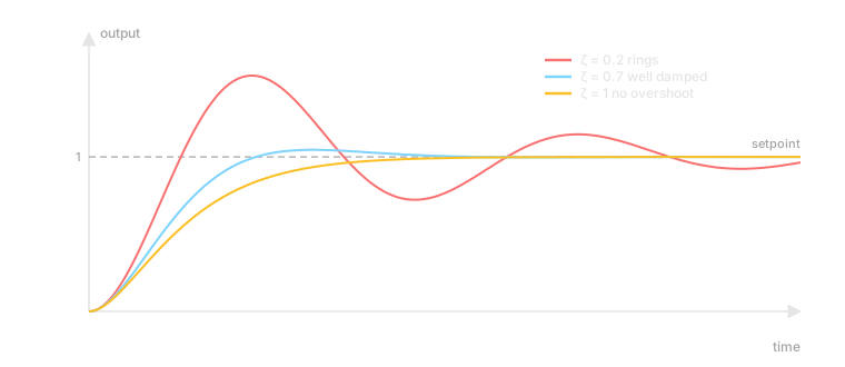
Figure 4. The same step for three damping ratios. Low damping overshoots and rings, $\zeta = 1$ never overshoots, and $\zeta \approx 0.7$ is the usual compromise: fast, with a small overshoot.

Low damping is fast but rings. High damping is calm but slow. Most practical tuning aims for something near $\zeta = 0.7$. The manufacturing circuit model uses this idea to tune control gain and adjustment lag, then checks physical WIP capacity separately. Adding unused storage alone does not change damping.

6. Discrete time and the z-plane

Many real loops don't act continuously. They act once per period: a paycheck, a weekly review, a controller scan cycle. For these, $s$ is replaced by $z$, where multiplying by $z^{-1}$ means "one period ago." A delay of $d$ periods is $z^{-d}$, and a running total (the discrete integrator) is $1/(z - 1)$.

The stability rule changes shape but not meaning. A discrete system is stable when every pole sits inside the unit circle, $|z| < 1$. A pole at $z = 0.4$ shrinks the error by 60% each period. A pole at $z = 1.06$ grows it by 6% each period.

Discrete time allows something continuous time can't: a deadbeat controller, which removes an error completely in a single step. Topping a checking account back up to its target on every payday is deadbeat control.

7. Delay: the dangerous part

Dead time, a delay between acting and seeing the result, is what destabilizes most real loops. The controller keeps pushing because it can't yet see that its last push worked. By the time the effect arrives, it has pushed too far, and the correction overshoots the other way.

Take the simplest discrete loop: each period, move a fraction $Ka$ of the measured error, where the measurement is $d$ periods old.

$$x[n+1] = x[n] - Ka\,\big(x[n-d] - 1\big)$$

With no delay, it's stable for $0 < Ka < 2$. With one period of delay, the characteristic equation becomes $z^2 - z + Ka = 0$, and stability needs $Ka < 1$. Every extra period of delay tightens the limit further.

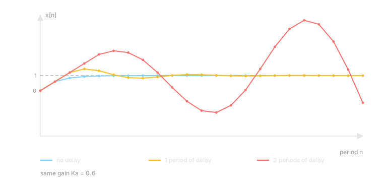
Figure 5. The same gain, $Ka = 0.6$, with three amounts of delay. With no delay it settles smoothly. With one period it rings and settles. With three periods the same gain is unstable, and the swings grow.

That's the whole argument behind "wait for the data before you react again." When a measurement is slow (ad attribution, payouts, a prediction's due date), the safe move is to lower the gain: react less, or react less often.

8. The practical layer

Real loops add a few things the clean math leaves out:

• Saturation. Actuators have limits: a valve can only open so far, and a budget can only spend so much. Drawn as a block with a flat-topped curve, saturation also works as a safety feature.
• Rate limits. These cap how fast an input may change, so one bad decision can't move the system far.
• Adjustable gain. The gain is tuned while running, often by a slower outer loop. It's drawn as a diagonal arrow through the block.
• Interlocks. These are hard stops that sit outside the control logic. On a plant, the safety system is separate from the process controller, and the operator can't edit it.
• System identification. Measure how the plant responds, at a fixed open-loop input, before closing the loop. You can't tune a gain you haven't measured.

Notation used in this section

Symbol	Meaning
$r, R(s)$	Reference, the setpoint
$y, Y(s)$	Output
$e, E(s)$	Error: reference minus measurement
$u, U(s)$	Actuation: the controller's output
$G, C, H$	Plant, controller, sensor transfer functions
$K$	A gain, often the adjustable one
$s$	Laplace variable (continuous time). $1/s$ is an integrator
$z$	Discrete-time variable. $z^{-1}$ is one period of delay, $1/(z-1)$ a running total
$e^{-sT}$, $z^{-d}$	Dead time of $T$ seconds, or $d$ periods
$\zeta, \omega_n$	Damping ratio, natural frequency

The other pages reuse letters for their own quantities (in the money article, $D$ is owner draws and $r$ is the savings yield). Each page defines its symbols where they first appear.

Where to go next

1. Money as a Control System: integrators, positive feedback, a deadbeat buffer and a delayed loop, applied to savings and a business.
2. Agent Autonomy as Loop Gain: adjustable gain, saturation, interlocks and an outer tuning loop, applied to AI agents.
3. A Circuit-Inspired Framework for Manufacturing Systems: second-order dynamics and damping on a production line.
4. Everything I Build Is a Control Loop: the short version, without the math.